Metadata
aliases: []
shorthands: {}
created: 2022-07-08 17:48:33
modified: 2022-07-11 10:33:34
Let's suppose that in our case, the shear zone is perpendicular to the
Our goal is to first approximate the velocities of the particles using the tanh function by fitting in Python. The shear zone can have a displacement from
def vel_estimator_func(coord, transition_rate, y_displacement, x_lin, x_quad, z_lin, z_quad):
    x = coord[0]
    y = coord[1]
    z = coord[2]
    return np.tanh(y_displacement + (y + x*x_lin + x*x*x_quad + z*z_lin + z*z*z_quad)*transition_rate)
Then we can define the shearing rate, aka the
def vel_estimator_func_derivative_y(coord, transition_rate, y_displacement, x_lin, x_quad, z_lin, z_quad):
    return transition_rate * (1 - vel_estimator_func(coord, transition_rate, y_displacement, x_lin, x_quad, z_lin, z_quad)**2)
Then optimizing will be easy using the curve_fit function from scipy:
import scipy
from scipy import optimize

fitParams, fitCovariances = optimize.curve_fit(
    vel_estimator_func, [coords[:, 0], coords[:, 1], coords[:, 2]], vs[:, 0])
The approximated values of gradient in the position of each particle is also easy to get here, in one fast step:
gradient_from_fit = -vel_estimator_func_derivative_y(
        [coords[:, 0], coords[:, 1], coords[:, 2]], *fitParams)
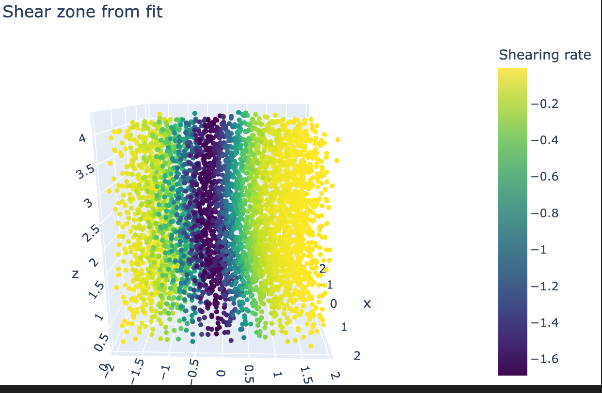
Then, if we use these gradient values as color in a scatter plot, we can visualize the approximated shear zone:
import plotly.graph_objects as go

fig = go.Figure(data=[go.Scatter3d(x=coords[:, 0], y=coords[:, 1], z=coords[:, 2],
                                   mode='markers',
                                   marker=dict(
    size=3, color=(gradient_from_fit),
    colorbar=dict(title="Shearing rate"),
    colorscale='Viridis',
    showscale=True))])
fig.update_layout(width=650, height=400, margin=dict(
    l=0, r=0, b=0, t=40), title="Shear zone from fit")
fig.show()
As we can see, it has a bent shape and it resembles the example seen in Determining the shear zone of split bottom sheared granular materials from simulation data.
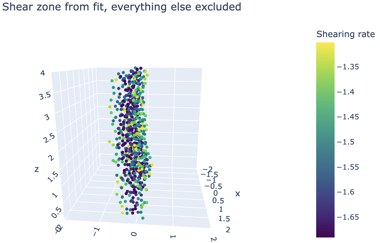
We can now also easily filter out the particles that are not in the shear zone, using just:
zone_filter = gradient_from_fit < -1.3
Where 1.3 is just an arbitrary threshold, it should be set by how much of the shear zone is to be included. In the January 2022 simulations, 1.3 seemed the best.
We can use zone filter like this, to only handle the points inside the shear zone:
coords[zone_filter]
gradient_from_fit[zone_filer]
# ...
With this, we can plot again:
fig = go.Figure(data=[go.Scatter3d(x=coords[:, 0][zone_filter], y=coords[:, 1][zone_filter], z=coords[:, 2][zone_filter],
                                   mode='markers',
                                   marker=dict(
    size=3, color=(gradient_from_fit[zone_filter]),
    colorscale='Viridis',
    colorbar=dict(title="Shearing rate"),
    showscale=True))])
fig.update_layout(width=650, height=400, margin=dict(
    l=0, r=0, b=0, t=40), title="Shear zone from fit, everything else excluded", scene_aspectmode='cube')
fig.update_layout(
    scene=dict(
        xaxis=dict(range=[-2, 2],),
        yaxis=dict(range=[-2, 2],),
        zaxis=dict(range=[-0, 4],))
)
fig.show()
To get this:
transition_rate is constant, the thickness of the shear zone is of constant width with respect to changes in spatial coordinates